How to Make a Google Sheets Header Row

On practically every spreadsheet I produce on Google Sheets, I use header rows.

It not only helps me ensure that I am putting the correct data in the correct column, but it also helps the individuals who will be viewing that data later.

In this tutorial, you’ll learn how to create a header row in Google Sheets and lock it to the top of the spreadsheet.

Summary – How to Create a Header Row in Google Sheets

1. Open your Google Sheets spreadsheet.
2. Fill up the blanks in row 1 with a description.
3. At the top of the page, click the View tab.
4. Select the Freeze option, then select the first row.

Our post continues below with more information, including screenshots, on adding a header row to a Google Sheets spreadsheet.

In Google Sheets, adding a header row makes it much easier to identify the information contained within a column. You can also keep that header row visible at the top of the spreadsheet while scrolling. To create a header row in Google Sheets, follow these instructions.

Spreadsheets can quickly become difficult to comprehend as more information is added. It becomes even more difficult when the information in your columns is substantially similar to that in other columns.

Creating a header row is one method to simplify this. Entering a description of the type of information included within a column makes it easier to modify and view the information.

After you’ve entered those explanations, you can select to freeze the top header row of the document. This allows you to continue scrolling down the spreadsheet while keeping the header row displayed.

The instructions below will show you how to add a header row to a Google Sheets spreadsheet.

Excel, Microsoft’s equivalent to Sheets, shares many of the same features. For example, our guide on producing tables in Excel demonstrates how to convert a selection into a table in that program.

How to Make a Google Sheets Header Row

The methods in this post were carried out on the desktop version of Google Chrome, but they will also work in other desktop browsers such as Firefox or Safari.

Step 1: Log in to Google Drive and open or create a new spreadsheet.

Step 2: In the A1 cell, type a description for the first column, then repeat for each other column in the spreadsheet.

In the figure below, for example, I have three columns. The text “First Name,” “Last Name,” and “Employee ID” will all serve as headers for the data contained in the remaining cells in those columns.

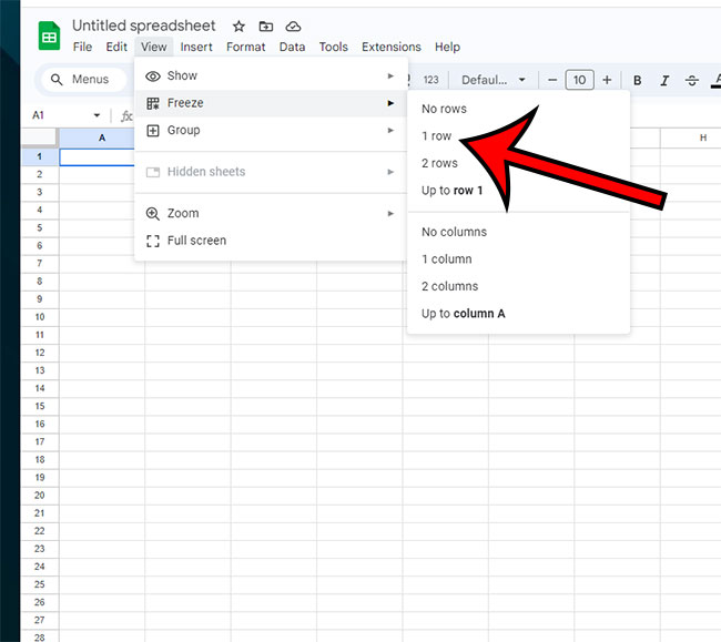
Step 3: At the top of the window, click the View tab.

Step 4: Select the 1 row option from the Freeze menu.

When you navigate down in your spreadsheet, the header row will remain frozen at the top, allowing you to simply enter the necessary information to each of your columns.

Because you now know how to create a Google Sheets header row, you will be able to use this skill to make your spreadsheets much easier to read and understand in the future, which your readers will much appreciate.

If you already have data in your spreadsheet’s cells, you may insert a new row at the top by right-clicking on the row 1 label on the left side of the window and selecting the Insert 1 above option. This will cause all of your data to be slid down one row.

If you frequently transition between Google Sheets and Microsoft Excel, read our guide on adding columns in Excel to learn about a quick and simple approach for totaling column values in a spreadsheet.

Header Rows in Google Sheets: Frequently Asked Questions

In Google Sheets, how do I make the first row a header?

If you want to transform the first row of your spreadsheet into a header, follow the methods outlined in our previous post.

You must first insert the headers for each of your columns into the first row’s cell, after which you can pick the View tab at the top of the window and choose to freeze the top row. This ensures that the data in the first row is visible when you navigate down through the spreadsheet.

In Google Sheets, how can I make a header?

The process for creating a Google Sheets header differs differently because it is a separate entity from the header row.

While a header row in a spreadsheet indicates the type of data in a column, a “header” in a spreadsheet will contain information such as page numbers, author name, corporate logo, or spreadsheet name.

In Google Sheets, go to File > Print and then click the Headers & Footers button on the right side of the window to create a heading.

You will be able to select the type of data to put in the header there. You can also choose Edit Custom Fields if you want to include data in the header for which no options are available.

How do I create a header row?

Adding a header row to your Google Sheets spreadsheet is as simple as inserting descriptive content into the spreadsheet’s top row.

While our article concentrates on freezing the top row to keep it visible and making it possible to print that row at the top of every page, merely inserting a description in the first row is often enough to make that row into a header row.

In Google Sheets, what is a header row?

If you’ve heard the word “header row” and aren’t familiar with it, you might be wondering what it means.

A header row in a spreadsheet is a row that contains an explanation of the data in the columns below it.

This header row is usually the first row in the spreadsheet.

By placing a row at the top of the spreadsheet that identifies the information in the cells below it, you can verify that you are putting the correct data in the correct place, reducing errors.

It is also advantageous to those who may be looking at your data because they will not have to try to figure out how you have ordered everything.

You can also freeze the header row to keep it at the top of the sheet as you scroll down. This makes it much easier to add new data to the correct location because you won’t have to continuously scrolling up to see the content in the header row because it will always be displayed.

While the majority of this article has focused on adding a header row to a blank spreadsheet, you may be wondering what to do when you want to include a header row at the top of a spreadsheet that already has data.

In Google Sheets, how can you insert a row above the first row?

If you already have data in your spreadsheet, there is a fair likelihood that it is in the first row.

It may appear at first that you will have difficulty generating a Google Sheets header row in this case, but there is really a quick series of actions that you can take to position a blank row above the existing text.

Step 1: Open your Google Sheets spreadsheet.

Step 2: On the left side of the window, select the row 1 heading.
choose the first row

Step 3: Right-click on the desired row number and select Insert 1 row above.

You should now have a blank row at the top of the sheet that you can fill with the information from your header row.

If you want to keep that row at the top of the sheet while scrolling down, repeat the previous steps.

More on How to Create a Header Row in Google Sheets

For many spreadsheets, you will almost certainly only want to freeze the first row.

When you freeze rows in a spreadsheet, make sure they stay visible when you scroll so you don’t enter data into the wrong column.

However, if your spreadsheet structure demands several columns or if you use more than one row to represent significant information, you may wish to freeze more than one row. If this is the case, you can opt to freeze rows up until the one currently chosen in your spreadsheet.

To choose a row, click the row number on the left side of the window. The same action can be used to pick a full column by clicking the column letter at the top of the sheet.

The View menu at the top of the window not only allows you to freeze rows, but it also allows you to hide or reveal gridlines, view formulas, and zoom in on your data.

While it lacks the variety of viewing choices provided in Microsoft Excel, many Excel users have considered Google Sheets to be a competent alternative to Microsoft’s premium spreadsheet application.

As a previous Excel user, transitioning to Google Sheets can be difficult.

While many of the application’s functions are easy to find, others, particularly the printing and viewing options, may require some practice until you become acquainted with them.

If there’s something you want to modify about the way your Google Sheet looks on the screen or when you print it, there’s probably a method to do it.

Familiarize yourself with the View menu and the File > Print menu, as that are where the majority of those options can be located.